Executive Summary
My project involves the analysis of word usage frequencies in the English language. This type of analysis has implications not only for critical fields of research, such as crypto analysis, speech recognition, and human-like artificial intelligence, but also for managing enormous data sets that are beyond the capacity of the typical computer. For this project, I developed algorithms for working with linguistic data sets involving billions of words, and doing so efficiently. I have also written code to collect new and original linguistic data sets. I hope some of the techniques I have developed might suggest approaches to other researchers attempting to handle similar large linguistic data sets.
To gather a representative data set of words in literature, I utilized data from the Google N-grams project which was compiled from about five million books. In addition, I developed code to compile my own data set from Twitter. I developed code to calculate frequency data from these two sources, and to analyze the similarities and differences between the two samples using C++, C Sharp, and R. My analyses take into consideration a wide range of variables involved in computer analysis of linguistic data, from how to determine what is a word, to weights of word frequencies over time, to spelling errors on Twitter, and even upper versus lower case.
Problem Statement
I began considering word frequencies out of curiosity about infrequently used words. I didn't initially appreciate how long it might take me to get answers, especially regarding comparative word usage frequency; however, it quickly became apparent that it would be much more complicated than the 30-line python program I had set out to write. So I began thinking about ways I could write code to efficiently analyze word usage frequencies. When I decided to develop this project for the Supercomputing Challenge, I was told that linguistic analysis would be too massive of an undertaking to tackle, and I was urged to downsize.
When performing linguistic analysis, immense amounts of data need to be processed and analyzed. The problem is that without specialized methods, computers cannot work with that quantity of data. This means that important questions in linguistics have not been tackled and/or adequately answered because the data sets are too unwieldy. As I delved into this project, I became fascinated not only with finding answers to my questions regarding word usage frequency, but with the challenge of writing code that could solve some of the problems with analyzing these large data sets. I decided to forge ahead.
The purpose of my project is to analyze the word usage frequency in English literature and in social media, analyze the differences between the data sets, and offer possible conclusions from those results.
Literature
The first part of this project is analyzing the word usage frequency in literature. Since I do not have the means to obtain a reasonable sample size of digitized books to process, I am relying on previous research done by researchers at Google. The Google N-grams project is a fascinating project, aimed at looking at the frequency of words or phrases over time (see Appendix A for an example). Google's data is built from about five million (roughly 4% of all books ever printed) digitized books. These books were sourced in libraries from about 40 universities worldwide (see Appendix B for more information). Google also excluded N-grams which appeared less than 40 times. We can assume that Google's data is independent: if books influence each other, it would be statistically insignificant with this large of a sample. We can assume that the data is random, since university libraries should have a sufficiently random sample of books. This is important, because it means that we can use a normal model for estimating the true proportions of data. Google has made the results of their research available to the public on the Google Books N-grams Viewer, as well as making the raw data available to everyone under the creative commons license. The sheer quantity of data is ginormous, something that only a large corporation like Google would have the resources to process. Thus, in order to make the raw data manageable, Google has subdivided the data into several categories: 1-grams, 2-grams, 3-grams, 4-grams, and 5-grams. 1-grams are single words or strings of characters which are not separated by a space, such as "Hello" or "3.1415". 2-grams are strings of characters which are separated by 1 space, like "Hello, World", or "Pi: 3.14159". The same pattern follows for the rest of the N-grams. The data is available to be downloaded on the google N-grams project page (see Appendix C for more information). For this project, I am limiting the scope to 1-grams, single words. The English 1-grams consist of 39 files, each containing 1-grams beginning with a different letter. The other files are for N-grams that do not begin with letters. Every file is in a consistent format, as shown in Figure 1.
	0'9	1797	1	1
	0'9	1803	1	1
	0'9	1816	2	2
	0'9	1817	1	1
	0'9	1824	4	4
	0'9	1835	1	1
	0'9	1836	2	2
	0'9	1839	8	4
	0'9	1843	2	1
	0'9	1846	3	3
	0'9	1848	1	1
	0'9	1849	2	2
	0'9	1850	3	3
	0'9	1851	5	4
	0'9	1852	2	2
	0'9	..	..	..
0'9 2008 43 36 This is from the "googlebooks-eng-all-1gram-20120701-0", which contains all the 1-grams beginning with the number "0". The first column is the 1-gram itself, followed by a tab, then followed by the year. The next two numbers are the number of occurrences and the number of volumes respectively for that year. This tells us that in 1851, the 1-gram "0'9" was used 5 times in 4 distinct volumes. Getting the frequency of this 1-gram is straightforward. Google provides a file with total counts for each year, containing the year, the total occurrences for that year, pages, and volumes. Figure 2 shows the corresponding total count for the year 1851.
1851 537705793 2787491 4021 So the frequency of the 1-gram "0'9" in 1851 was \(5 / 537705793\), which is roughly \(9.299x10^{-9}\).
The size of all the data combined is almost 30 gigabytes, more than the amount of RAM most computers have. Some files, like the file with 1-grams starting with "A", are over 1.67 gigabytes alone. There is just too much data to all be handled at the same time. There is a simple solution to this, and that is to pre-process every file, compressing it down to just the information that is needed. One huge memory optimization can be made that drastically reduces the computation time, which is compressing the data from multiple years into just one line and only keeping the data that is needed. Since the focus of this project is to find the frequency of a word - as opposed to the frequency over time - an algorithm must be used to compress the frequencies from multiple years into just one year. There are a handful of methods for computing this; one such method would be to simply take a raw mean of the frequency for each year. However, since the frequency data from this will be compared against data from today's Twitter feeds, it makes the most sense to do a weighted mean, with more recent years weighed more heavily. The best way to do that is by weighing each term exponentially, as defined by the following formula:
$$\mu_n=\alpha F_n + (1-\alpha) \mu_{(n-1)}$$ $$\alpha = \frac{2}{n - 1}$$Where \(\mu_0=F_0\), and \(F_n\) is the frequency from index \(n\). It can be implemented very easily with the following code:
int N = frequencies.size();
double Mu;
if (N > 1) {
	Mu = frequencies[N - 1];
	double k = 2.0 / ((double)N + 1.0);
	for (int i = N - 2; i >= 0; i--) {
		Mu = (double)((frequencies[i] * k) + (Mu * (1 - k)));
	}
}
else {
	Mu = frequencies[0];
}
worddata wdata = { currentWord, Mu, previousRecentCount, previousRecentTotal };
localWordBank.push_back(wdata);
Where frequencies is a vector, composed of the frequencies for each consecutive year.
frequencies.push_back((double)data.occurrences / (double)totals[data.year].matches);The most recent count and most recent total are also saved, for estimating the standard deviation later. This optimization compresses the data massively, for example the "A" file compressed by a factor of almost 50x, going from 1.67 gigabytes to just 33.7 megabytes.
A large factor in the computation time for this data is the reading of the file into memory and parsing it. The following code is used to read in a file:
inputData data;
std::ifstream fIn(PATH + FILEPREF + letterScan);
while (fIn >> data.name >> data.year >> data. occurrences >> data.volcount) {
	...
}
And the inputData structure is defined as:
struct inputData {
	std::string name;
	int year;
	double occurrences;
	unsigned long long volcount;
};
This cannot be optimized very much. Even the C++ Boost Library does not provide much of a boost to the speed. This is mainly because of parsing the numbers. Precompiling the data into a smaller format circumvents this problem, by only requiring the intensive parsing to only be run once, allowing for easier tweaking of other parts of the code later on. The total size of all the Google data is almost 30 gigabytes, while the compiled data is just a mere 450 megabytes. The N-gram data for "0'9" is 168 lines, but with precompiling it is compressed down to just one line, as shown in Figure 3.
0'9 7.48321e-09 43 19482936409 I had a small bug early in the writing of the code, where I accidentally weighed the frequencies in the wrong direction, weighing ancient frequencies much more than today's frequencies, which yielded some interesting results. While words like "The", "God", and "It" remained much the same in terms of frequency, some other words were reported as much more common. Examples are words like "Presbyters", "Michelangelo", and "Vasari" (See Appendix D). A lot of words you might find in 17th and 18th century texts appear at the top of the list like "Committee", "Lord", "Parliament", "Medals", and "Viator" also appeared near the top due to the incorrect weights.
The most significant optimization is allowing the program to utilize almost all of the CPU by multithreading the application. Since the bottleneck is caused by the parsing of each row of data itself, this optimization also allows more of the available hard drive read/write speed to be used. My computer has an Intel 6th generation core i7 processor, with 4 physical cores and 8 virtual cores. When multithreading the application, the program will only use 7 threads, one for each virtual core, leaving 1 core for the system and other processes on my computer, as follows:
// assignment lock
std::mutex Lock;
// Number of processing threads
const int NUMTHREADS = 7;
// Keep track of threads
std::vector<std::thread> threads(NUMTHREADS);
// ...
void Preprocess(std::string name, int delay) {
	// Avoid coordination issues by staggering
	Sleep(delay * 1);
	// Create a bank of data which we will output to the preprocess file
	std::vector<worddata> localWordBank;
	// Until we have processed every file, get a new one an process it
	while (true) {
		// ... Read each file line by line and process it
	}
	std::cout << name << " ending - no more assignments" << std::endl;
}
// ...
int main()
{
	// ...
	for (int i = 0; i < NUMTHREADS; i++) {
		threads[i] = std::thread(Preprocess, "T" + std::to_string(i), i);
	}
}
And of course, the threads have to be coordinated, so each thread processes a new N-gram file:
class threadCoordinator {
public:
	static char getAssignment() {
		if (FileIndex == FileIndex _len) {
			// We have reached the end, finally. Tell the threads to die quietly.
			return '-';
		}
		// Return next data file in queue, and increment afterwards so that a new file is queued
		return FileIndexes[FileIndex++];
	}
};
After precompiling, the data can now be worked with much more easily, making the process of analyzing the code more straightforward to work with. Processing the data to find out the frequency of N-grams is one thing, but verifying that the N-grams are words is a completely different story. One method which I explored was verifying if an N-gram was a word based off the vowel-to-consonant ratio. That method is reasonable and filters out many non-words. However, it is not even close to 100% accurate, and it does not account for the odd word in another language or semi-random strings of characters that could be caused by Optical Character Recognition (OCR) error. The optimal solution is to use an English wordlist, and check if each N-gram is present in the wordlist. This is a much better solution because at least every N-gram in the output file will be a word. The only potential error with a wordlist would be caused by missing words in the wordlist; however, this is fairly unlikely. I am using an alphabetized wordlist that I compiled a year or two ago as a side project, which contains over 293,000 words. Since the wordlist is alphabetized, the process of checking if N-grams are words can be optimized significantly by using a binary search algorithm. The binary search algorithm places a cursor at the middle of the dictionary, checks if the N-gram should be above or below it, then repeats with the smaller chunk. A standard search algorithm would have to go through the dictionary one item at a time and check for equality, with a worst-case scenario of \(O(N)\), where \(N\) is the total number of items in the array. A binary search algorithm, on the other hand has a worst-case scenario of \(O(\lfloor log_2 N\rfloor+1)\), meaning that the worst-case scenario for a wordlist of 293,000 is only 19 comparisons. About 50% of the 1-grams that are words will take 19 comparisons to verify, however that is still significantly better than searching every word in the wordlist.
The processor program works much the same as the preprocessor program, with 7 threads working simultaneously to process each file. One difference is that the processor only processes a fraction of the data, using the precompiled data. Another difference is that it first identifies N-grams that are words, and then only processes those N-grams. The program finishes by sorting the words in order of least frequent to most frequent, then writes that data to a file, in a consistent format as shown in Figure 4.
	Bogarted	1.91368e-10	1	19482936409
	Shtupping	1.9677e-10	4	19482936409
	Strawweight	2.1138e-10	1	19482936409
	Cannibalising	2.1536e-10	1	19482936409
	Ivermectins	2.17086e-10	1	19482936409
	Malfeasant	2.179e-10	1	19482936409
	Archaeobotanist	2.19215e-10	4	19482936409
	Countersue	2.19712e-10	3	19482936409
	Bandmate	2.2011e-10	7	19482936409
	Hematal		2.22227e-10	1	19482936409
Stealthed 2.22556e-10 4 19482936409 The frequency data has produced interesting results. R is used to graph the data, using the following code:
plot(x, freq, type="p", main="Literature Word frequency", xlab="Word", ylab="Frequency", pch=20)The result is a seemingly exponential distribution, as shown in Figure 5.
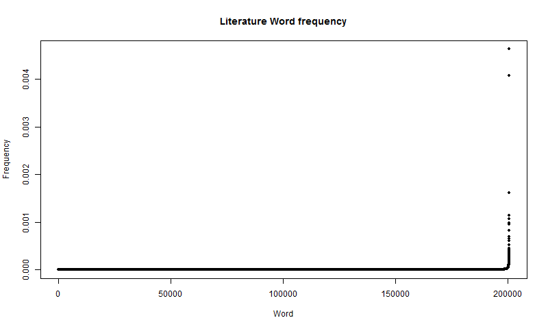
The distribution appears to be completely flat for the majority of the data points, up until the very end, where it shoots up vertically. There are two data points at the top. Those are "I" and "The". These words are very common and irreplaceable in English, so it makes sense that they would be so much more common than all other words. This also tells us that in literature nearly 1% of all N-grams are either "I" or "The". After these words, there is a severe drop-off, going from a frequency of nearly 0.5% to just a little over 0.1%. That 3rd most frequent word is "And", which again, is a word in English that, while hard to replace, is easier to replace than "I" or "The", which may explain the drop-off to a certain extent. This distribution is interesting, but more detail is needed to see what is going on in the rest of the graph, not just the top few words. We can achieve this by taking the plotting the \(log(Frequency)\), using the following code:
logfreq = log(freq)
plot(x, logfreq, type="p", main="Log Literature Word frequency", xlab="Word", ylab="Log(Frequency)", pch=20)
The resulting distribution is shown in Figure 6.
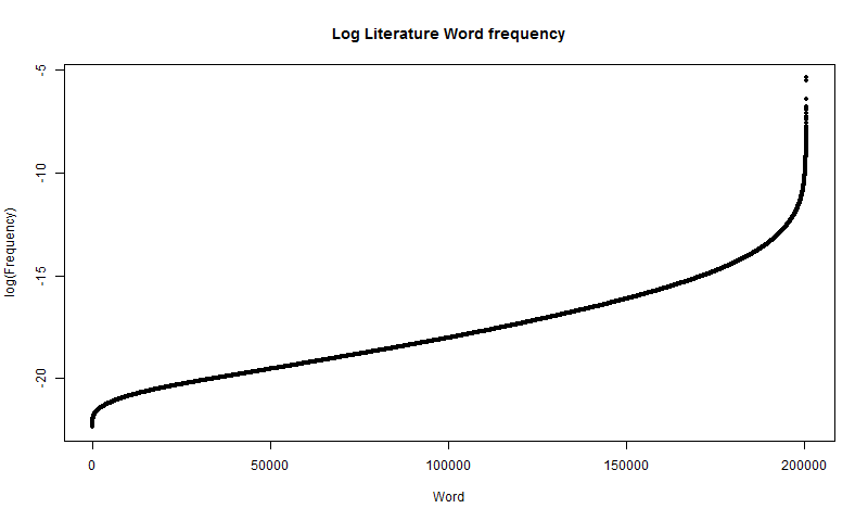
This display provides even more insight than the first. Mainly, if word frequency were exponential, this would be a linear distribution; however, it is not. At the left tail, an exponential graph would overestimate, and at the right tail, it would underestimate. However, in the middle, from about the 1,000th word to the 175,000th word, it is relatively linear. Of course, that means that it would be an exponential distribution within this interval.
The raw count for the most recent year and total for that year are written to the precompiled file, and up until now they haven't been used. Each year a count is stored out of a total; that count is a proportion. The reason the raw count is written to the file is for estimating the standard deviation of the proportion, using the following formula:
$$SD(\widehat{freq})=\sqrt{\frac{freq\cdot(1-freq)}{n}}$$Where \(\widehat{freq}\) is the sample proportion, and n is the total count for that year. The following code is used to compute the estimated standard deviation and graph the standard deviation:
counts <- as.vector(processed[["V3"]])
totals <- as.vector(processed[["V4"]])
recentfrequencies <- counts / totals
standarddeviation <- sqrt((recentfrequencies * (1 - recentfrequencies)) / totals)
plot(x, standarddeviation, type="p", main="Recent Standard Deviation in Literature Word frequency", xlab="Word", ylab="SD(freq)", pch=".")
Which produces a plot similar to the literature distribution plot, as shown in Figure 7:
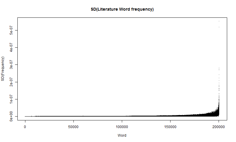
This plot follows much the same pattern as the distribution plot, appearing to be exponential. The main difference is towards the right-hand side, the plot thickens. This is most likely caused by tiny fluctuations in the data. Like with the distribution plot, it can be good to observe the log plot as well, which is graphed using the following code:
plot(x, log(standarddeviation), type="p", main="Log Recent Standard Deviation in Literature Word frequency", xlab="Word", ylab="Log(SD(freq))", pch=".")
par(new=T)
plot(x, log(frequency), type="p", xlab="", ylab="", axes=F, pch=".", col="red")
This code both graphs the \(log(SD(\widehat{freq}))\) and graphs the \(log(freq)\) plot from before on top of it, in red, for comparison, as displayed in Figure 8. Note: the red is drawn over the log plot, not using the same y-min and y-max values for rendering, so the graph is a little miss-leading. The red data is there to compare the form of the data.
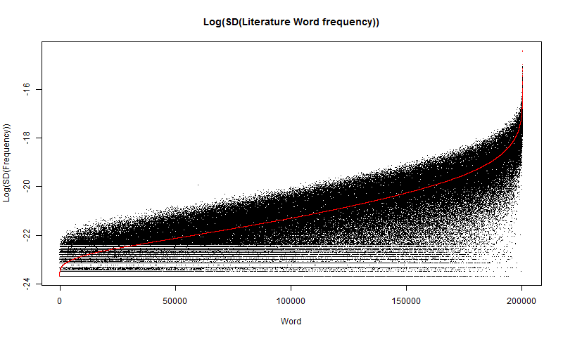
This distribution is quite intriguing. It does follow the log plot the same way it follows the regular distribution plot, however it is very noisy. Again, the noise is probably caused by small fluctuations in the data. But there is one curious aspect, which is that there are bands at the bottom of the plot, which seems to start abruptly. I think they are caused by numbers being too small for a computer to calculate accurately, leading to rounding which causes bands to form.
Another graph to look at, is the relative standard deviation. This can be done by taking \(SD(\widehat{freq})/freq\), as shown in Figure 9.
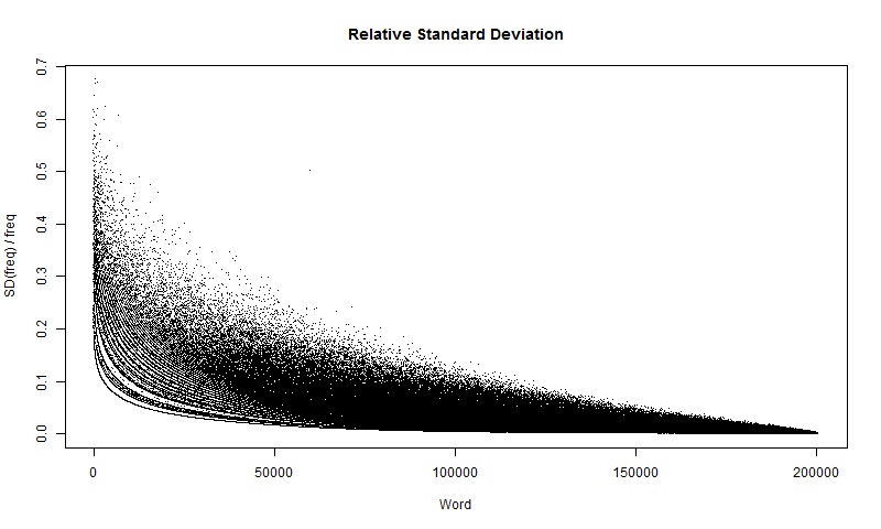
I could create a 95% confidence interval around a word with the following formula:
$$freq \pm 1.64*SD(\widehat{freq})$$Where the number \(1.64\) comes from the critical Z-value. Figure 9 shows that even though the words with higher frequencies have a higher standard deviation, they have a smaller relative standard deviation. On the contrary, words with lower frequency and lower standard deviation also have higher relative standard deviation.
The second part of the project is to look at the frequency of words used in social media. I used Twitter as my data source, mainly because Twitter is the only social media I have experience with, and it has an Application Program Interface (API), which allows me to get the data I need. N-gram data isn't available for Twitter the same way it is for literature, so I also had to count the N-grams (specifically 1-grams) myself. The first part is getting a sufficiently large sample of tweets. Thankfully, the Twitter streaming API is extensively documented, and thus straightforward to access. I specifically used the "GET statuses/sample" API, which returns a random sample of all tweets in real time. I wrote the program to collect this data in C#, because it has a good library for working with the Twitter API, specifically the open source library, Tweet Invi. The implementation is as follows:
// Initiate Stream
var stream = Tweetinvi.Stream.CreateSampleStream(); // Have to call Tweetinvi.Stream explicitly because `Stream` interferes with System.IO
stream.StallWarnings = true;
stream.TweetReceived += (sender, args) =>
{
	// ...
}
Inside the brackets is code keeping track of statistics such as which language each tweet is in or the length of the tweet (see Appendix E). If the language of the tweet is English, then it is added to an array of tweets. I experimented with using a custom algorithm to identify the language of a tweet. Ultimately, I decided that the language tagging that Twitter does is most accurate, since the Twitter developers have put substantial time into language identification. To conserve on RAM, the tweets are flushed every 1,000 tweets, putting those one thousand tweets from the array onto the hard drive, then clearing the array. The application writes the data to a file, and to keep one tweet per line, the newlines are replaced with \uE032, which is a Unicode character in one of the special use planes, meaning it is safe to assume that it will never appear in a tweet. Therefore, they make a great solution for compressing a multi-line tweet into one line in a file without losing data.
This API feature is rate limited, so it takes a substantial amount of time to get a large sample of Tweets. An average of 40 Tweets per second is streamed to my client; of that, only about 12 tweets are usable. At this rate, it takes about a day to get a sample of 800,000 Tweets. I considered ignoring the re-tweets that are streamed; however, they should not cause any interference with duplicate Tweets, and would just cause it take longer to get a reasonable sample size. I also considered the fact that a lot of Twitter users misspell words in their tweets; however, trying to predict what word they meant risks errors which would hurt the accuracy of the frequencies. Unfortunately, using two streams does not half the time required, because the same tweets are streamed to each client. I am using a sample size of 800,000 tweets, which is smaller than I would like; however, it provides a large amount of insight. The algorithm for analyzing the Twitter data is straightforward. Since I am only concerned with N-grams which are words, I can create vector with counts for N-grams based off the dictionary, which I use to verify if an N-gram is a word. If I were interested in N-grams which were not words, then I would have to assemble the N-gram database while processing the tweets. That would increase the computation time massively because first I would have to search the database to see if the N-gram already exists, then add to its count; otherwise I would have to write another algorithm to place it alphabetically in the database. Again, alphabetizing is important because it allows me to use a binary search algorithm for finding words within the database, then adding to their counts. Building the database based off the dictionary is also more efficient because it is already alphabetized. I am using the following algorithm to process the raw data:
while (std::getline(fileIn, row))
{
	// Replace \uE032 with a space, so that the words on either side of it are counted as 1-grams
	std::replace(row.begin(), row.end(), '\uE032', ' ');
	// Split the Tweet into 1-Grams
	std::vector<std::string> words = split(row, ' ');
	std::string word;
	for (int i = 0, l = words.size(); i < l; i++) {
		word = words[i];
		// Transform the N-gram to lowercase. That way "The" and "the" are both counted
		std::transform(word.begin(), word.end(), word.begin(), ::tolower);
		// Find the index of this N-gram in the dictionary. A custom binary search algorithm is used because the binary search algorithm in the STL returns a binary value
		auto it = binary_find(dictionary.begin(), dictionary.end(), word);
		// Check to make sure the N-gram is in the dictionary. dictionary.cend() is returned if the N-gram could not be found
		if (it != dictionary.cend()) {
			// Determine the index in the dictionary
			int index = std::distance(dictionary.begin(), it);
			// Add to the count
			counts[index]++;
			// This could also be gotten from summing the counts vector at the end, however this is more efficient
			totalWords++;
		}
	}
}
This counts all the 1-grams that are words. Putting each 1-gram into lowercase is very important to get an accurate frequency. It accounts for the both uppercase and lowercase words, like "The" and "the", as well as counting the people who tweet in all caps like "THE" or the typos like "THe". Originally, I was just counting the 1-grams that were in the same form as the dictionary, which meant only uppercase words were counted, and that yielded a frequency of 0.50% for the 1-gram, "What". However, once I implemented the case changes, the frequency of "What" dropped down to 0.37%. Of course, not all words in the dictionary are used on Twitter, so a lot of 1-grams in my database show up as having 0% frequency. That is irrelevant to my sample, and they are disregarded. On top of that, any words which haven't appeared at least 5 times are ignored (the same way Google excluded N-grams with a frequency less than 40) since there is not enough data to accurately estimate the frequency. The frequencies are calculated after the N-gram database is assembled:
std::vector<worddata> words;
for (int i = 0, l = dictionary.size(); i < l; i++) {
	if (counts[i] < 5)
		continue;
	dictionary[i][0] = toupper(dictionary[i][0]);
	worddata wdata = {dictionary[i], (double)counts[i] / (double)totalWords, counts[i]};
	words.push_back(wdata);
}
SORT(words);
The same sort algorithm is used for sorting the data that is used in the Literature code. R is used again to graph the distribution, using much the same code as for the literature graphs:
plot(x, freq, type="p", main="Twitter Word frequency", xlab="Word", ylab="Frequency", pch=20)The resulting frequency distribution is similar to the literature data, as shown in Figure 10.
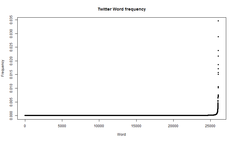
The first thing to notice is that it is remarkably similar to the distribution of words in literature, in the sense that it appears to be exponential, with most words being infrequent. However, with the literature data, there are over 200,000 1-grams which are words. In the Twitter data, however, there is only a vocabulary of just over 26,000 words. This is partially due to my lack of data, but also because a lot of words that are used in literature are outside of the vocabulary used by most Twitter users. Again, it is better to look at the log graph of the data, which is produced with the following code:
logfreq = log(freq)
plot(x, logfreq, type="p", main="Log Literature Word frequency", xlab="Word", ylab="Log(Frequency)", pch=20)
The resulting distribution, however, is different than the literature data, refer to figure 11.
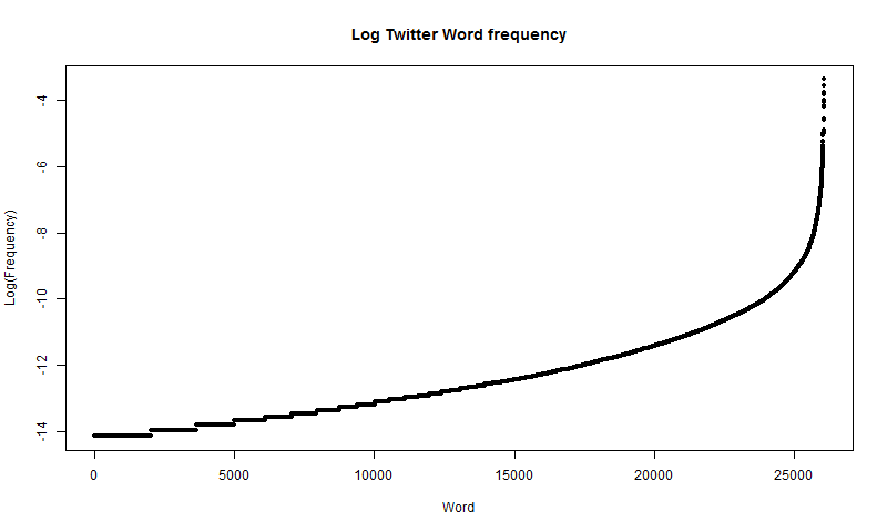
This distribution is significantly different than the literature data. Again, however, the data is roughly linearly distributed for most of the graph (of course a linear distribution on a log plot means that the data is exponentially distributed), but it curves up steeply at the right edge of the graph. One thing to notice about the log plot is that there are clear bumps (steps if you will) on left edge of the graph, which does not happen on the literature data plot. This is caused because there are numerous words that have appeared 5 times (anything less than 5 was disregarded), and thus have the same frequency, causing a flat section on the graph. This could be helped with more data. In the case of the literature data, the frequencies are derived from the moving average over multiple years, making it almost impossible for two words in the literature data to have the same frequency. Something else to notice about the two distributions is that the Twitter log graph looks a lot like the right half of the literature log graph. Figure 12 shows the two side by side for comparison.
If more data was readily available, the \(log(Frequency)\) for the Twitter data might match that of the literature data more at the left tail.
The program for compiling the Twitter data also has outputted the raw counts. Again, that can be used to estimate the standard deviation, \(SD(\widehat{freq})=\sqrt{\frac{freq*(1-freq)}{n}}\). The following code is used to compute and graph the standard deviation, with the frequency plot drawn on top of it in blue for comparison:
plot(x, sqrt((v * (1 - v)) / total), type="p", main="Twitter Word Frequency Standard Deviation", xlab="Word", ylab="SD(Frequency)", pch=".")
par(new=T)
plot(x, v, type="p", xlab="", ylab="", axes=F, pch=".", col="Blue")
The standard deviation plot produces a plot very similar to the frequency plot, as shown in Figure 13. Note again, that the frequency in blue is not at the same scale as the standard deviation data, and is only there for comparison.
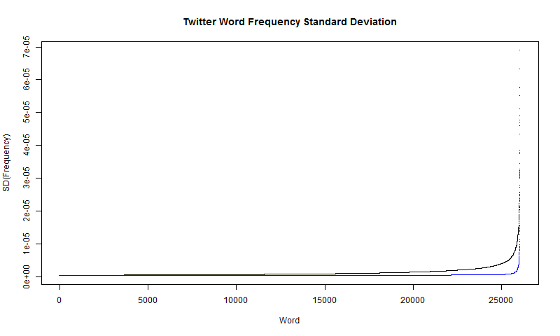
Like the literature data, the \(SD(\widehat{freq})\) plot seems to follow an exponential curve. The main difference, is that it appears to be much less noisy. I attribute this to having less data. The standard deviation plot also follows a similar form to that of the frequency plot. This of course means that when it comes to estimating the true frequencies, it is more accurate with the less frequent words. However, since the less frequent words also have smaller frequencies, it is important to again look at the relative frequencies. The following code is used to generate the relative frequency graph.
plot(x, sqrt((v * (1 - v)) / total) / v, type="p", main="Relative Frequency", ylab="SD(frequency) / frequency", xlab="Word", pch=".")The relative frequency graph for Twitter, however, is much different than the relative standard deviation plot for Literature, appearing to be almost linear, as shown in Figure 14.
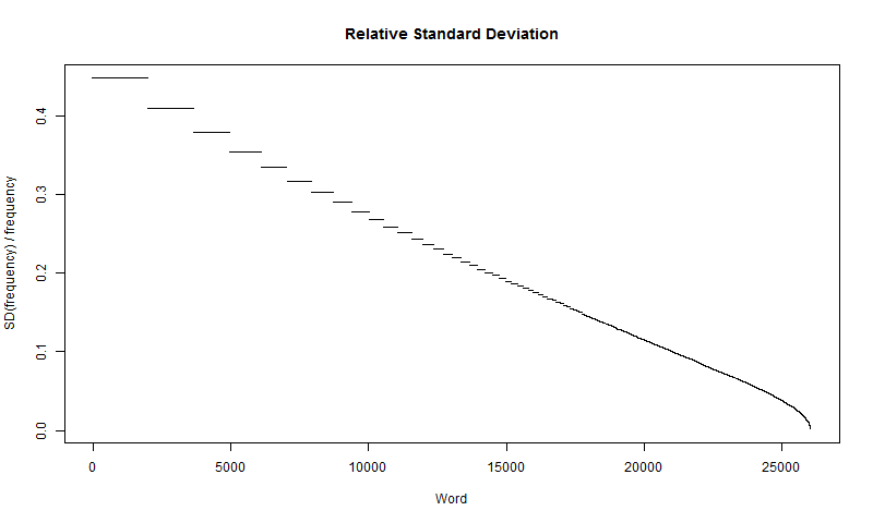
This shows how the standard deviation of the less common words is up to about 40% of the frequency of that word. It also shows that more frequent words, while having higher frequencies, have lower relative frequency.
Another difference between the literature and Twitter data sets is which words are most common. In literature, the most common words in descending order are: "I", "The", "And", "But", and "God". However, on Twitter, the most common words in descending order are: "The", "To", "A", "I", and "You". "And", while being the third most common word in literature, is the sixth most common on Twitter. On Twitter, "God" is the 186th most common word. Again, this makes sense because there is a lot of sacred writing in literature. Conversely, on Twitter, religion is not nearly as common a theme. Instead of religion, a very common topic on Twitter is politics. "Trump" is the 90th most common 1-gram on Twitter.
Conclusion
I began by processing the N-gram data for literature provided by Google. I sorted through that data, discarding non-words and computing an overall frequency from multiple years into one frequency value. Then I used that data to find out which words are more common than others. I also analyzed the distribution of the frequencies in depth. On top of that, I also computed the standard deviation of the proportions, providing insight into how far off the true frequency of a word is from the predicted frequency.
From my analyses of the literature data, I found that a small handful of words are much more common than the rest of the words. This makes sense, because some words in English are hard to replace. Also, in the case of literature especially, an effort is made to use more varied vocabulary. But literature is only one place where English is used. Analyzing word frequencies on Twitter provides an important window onto contemporary everyday use of language. Since N-gram data for Twitter is not available, I had to write a program from scratch to collect a large sample of tweets. I then compiled the tweets, counting up the 1-grams and excluding the non-words. I used the same processes to evaluate the Twitter data that I did with the literature data, analyzing the frequency distribution, and computing the standard deviation for the sample. The major difference between word usage on Twitter and in literature is that there are more high frequency words on Twitter as opposed to literature, in which there are more low frequency words. The sample from Twitter also has a much smaller vocabulary of words. This confirms what English teachers claim, that everyday language, such as that used on Twitter, tends to rely on a smaller range of vocabulary. Furthermore, the tweet-length constraint most likely compels people to use shorter words and, therefore, fewer different words.
I have developed specialized methods for working with the massive amount of data required for linguistic analysis. I was able to apply these techniques to two very different data sets, one of which I innovated methods for gathering. I explored a range of approaches, from multithreading to RAM conservation to developing more efficient algorithms for searching. With these techniques, I was able to answer my original questions, carry out the purpose of this project, and answer questions that came up along the way. I hope some of the techniques I have developed may be of use to others pursuing similar research.
I plan to continue my work on this project. One major issue which I would like to address is the sample size discrepancy. The Google N-gram data counts over 19 billion 1-grams in 2008 alone, and has N-gram data going back centuries. However, for the Twitter data, I only have 7 million 1-grams, from a 1-day sample. The Twitter data set provided a starting place for comparison but difference in sample sizes led to some complications with the data. Although processing Twitter data sets is time-consuming, I plan to continue increasing my Twitter sample size, so that I can further analyze and compare these two data sets.
Acknowledgements
I would like the opportunity to thank my English teacher, Mrs. Bethel, for unknowingly inspiring me to take on a humongous linguistics project. I would also like to thank my project mentor, Jim Mims, who always offered helpful advice for where to go with my project. And lastly, I would like to thank my sponsor and mentor, Kevin Fowler, who's positive attitude has fueled me in my endeavors.
Citations
Trampus, Mitja. "Evaluating Language Identification Performance." Twitter Blogs, Twitter, 16 Nov. 2016, blog.twitter.com/2015/evaluating-language-identification-performance.
Jean-Baptiste Michel*, Yuan Kui Shen, Aviva Presser Aiden, Adrian Veres, Matthew K. Gray, William Brockman, The Google Books Team, Joseph P. Pickett, Dale Hoiberg, Dan Clancy, Peter Norvig, Jon Orwant, Steven Pinker, Martin A. Nowak, and Erez Lieberman Aiden*. Quantitative Analysis of Culture Using Millions of Digitized Books. Science (Published online ahead of print: 12/16/2010) http://science.sciencemag.org/content/331/6014/176
Apendicies
Appendix A:
The Google N-grams project focused on analyzing the trends of N-grams over time. One of my favorite examples is graphing the trends in the frequency of "Great War" (blue), "World War I" (red), and "World War II" (green), as shown in Figure A1. 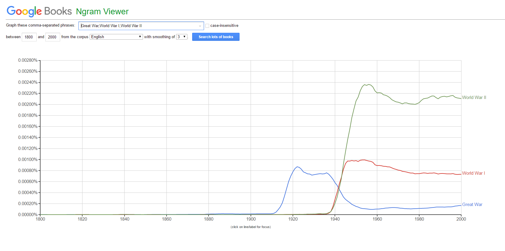
This really exemplifies how no one thought another massive war would happen, until about 1939, when authors really started referring to word wars with numbers.
Appendix B:
Google used OCR to digitize about 15 million books from about 40 university libraries. Of this 15-million-book sample, five million were selected to create the N-grams database, based off of OCR quality.
Appendix C:
While it works to download the N-grams data by hand, this is a computational challenge, and automation is always the way to go. I wrote the following shell script to download the data:
#!/bin/sh
LETTERS=(0 1 2 3 4 5 6 7 8 9 a b c d e f g h i j k l m n o p q r s t u v w x y z other pos punctuation)
CORPUS=eng-all
VERSION=20120701
cd ../data/
for i in "${LETTERS[@]}"
do
	URL="http://storage.googleapis.com/books/ngrams/books/googlebooks-$CORPUS-1gram-$VERSION-${i}.gz"
	echo "Downloading $URL"
	curl -O $URL
done
echo "Unziping..."
gunzip *.gz
URL="http://storage.googleapis.com/books/ngrams/books/googlebooks-$CORPUS-totalcounts-$VERSION.txt"
echo "Downloading $URL"
curl -O $URL
echo "Done"
Appendix D:
Some words appear more common with a weighted average in one direction, but appear as virtually non-existent when weighed from the other direction. One example is "Presbyters", which was common a few centuries ago, however is rarely used today. The historical data is plotted in Figure A2.
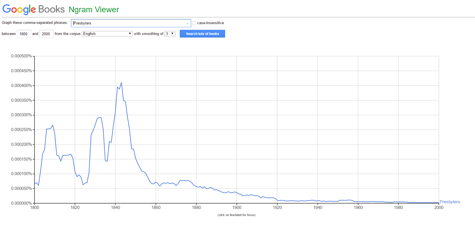
As is clear, this word would benefit greatly from being weighed with older data as more relevant.
Appendix E:
Twitter is susceptible to time zones. Sometimes English is the most common language on Twitter, however at night for us, Japanese becomes the most common language on Twitter. A pie chart with the number of tweets for each language is shown in Figure A3:
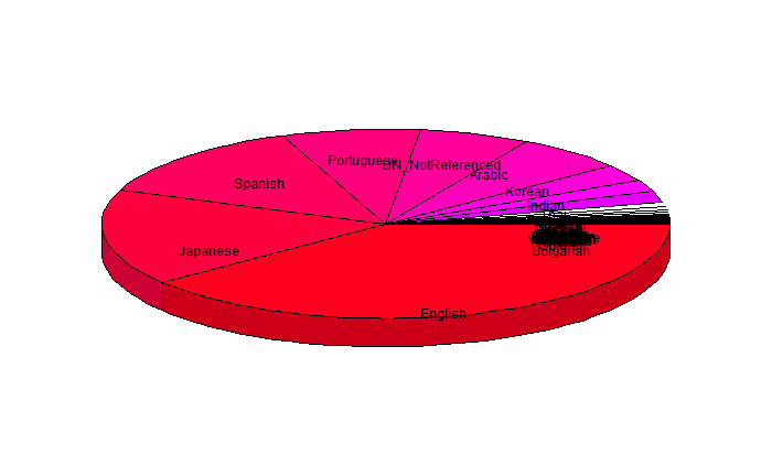
This is the result from a sample I took in the early morning mountain time, and English is clearly the most common. The slice labeled "UN_NotReferenced" corresponds to tweets which are not long enough to be accurately tagged as a language. While English is the most common language in this sample, Figure A4 shows the results of a sample taken over night our time.
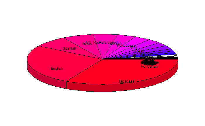
In this sample, Japanese is the most common. Interesting however, "UN_NotReferenced" is still about as common.
Code
You can view the sourcecode on: